MC/SA in GSAS-II
Introduction:
In these exercises you will use GSAS-II to solve the structures of 3-aminoquinoline and α-d-lactose monohydrate from powder diffraction data via Monte Carlo/Simulated Annealing (MC/SA). The data sets were kindly provided by Peter Stephens (SUNY StonyBrook) and were originally collected on NSLS beam line X3b1. The MC/SA technique is needed in these cases because as you will see the data does not extend very far in 2Θ so one cannot use charge flipping to solve them. The steps for each begin with peak selection and fitting, then indexing to identify the lattice parameters. A Pawley refinement is used to obtain a set of structure factors needed for the MC/SA runs. We will use previously developed models for the two molecules; I used the freeware program Avogadro (http://avogadro.cc/wiki/Main_Page) to create them.
If you have not done so already, start GSAS-II.
Step 1. Import powder data for 3-aminoquinoline
1. Use the Import/Powder Data/from GSAS powder data file menu item to read the data file into the current GSAS-II project. Change the file directory to MCsimanneal/data to find the file; you may need to change the file type to All files (*.*) to find the desired file.
2. Select the Quinoli.gda data file in the first dialog and press Open. There will be a Dialog box asking Is this the file you want? Press Yes button to proceed.
3. Select the BNL-I.instprm instrument parameter file in the second dialog and press Open. You’ll have to change the file type to *.instprm (GSAS-II instrument parameter file). The powder pattern will immediately appear.
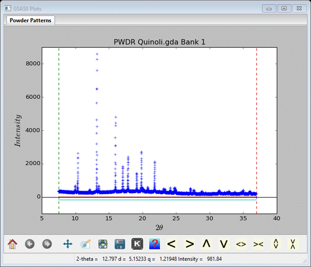
Notice that the pattern extends only to a minimum d-spacing of ~1.81Å; this is not far enough to use charge flipping which needs 1Å or better.
Step 2. Peak picking & fitting
Next you need to select limits so that ~20 peaks are selected for indexing; go to Limits and choose 9-25° 2Θ. Next go to Peak List and pick all the peaks you can see between the limits. This is most easily done by hand as the Auto search routine gives a lot of spurious peaks for this rather noisy and weak data; I picked 21 peaks, skipping a few very weak ones. Then use Peak Fitting/PeakFit to fit them (it will ask to save the project; I called it ‘2-amino’). You will need to refine at least X & Y in Instrument Parameters along with pos & int in the Peak List to get a reasonable fit suitable for indexing.
Step 3. Indexing
Next go to Index Peak List and do Operations/Load/Reload to set up the peaks for indexing. Then go to Unit Cells List for indexing. The most likely Bravais lattice for these small organic molecules is either Orthorhombic-P or Monoclinic-P; you can try both and see what comes out (Hint: it’s Orthorhombic-P). Click on Cell Index/Refine/Index Cell. The correct unit cell should almost immediately appear with an M20 ~370 with a=7.748, b=7.650, c=12.736, Vol=755.01. NB: your solution may have a & b switched. Do Cell Index/Refine/Copy Cell; you can then try various space groups. Press the Show HKL positions to see the lines with extinctions (Hint: it’s P 21 21 21). Under the General tab, change the space group to P 21 21 21. You can then do Cell Index/Refine/Refine Cell to improve the lattice parameters with M20 ~380. Finally do Cell Index/Refine/Make new phase to create the phase; I named it 3-aminoquinoline.
Step 4. Setup for Pawley refinement
There are a number of steps that must be done in preparation for a Pawley refinement after having completed the unit cell indexing and new phase creation. These cover two things: one is to prepare the powder pattern (reset limits, etc.) and the other is to prepare the phase for the refinement.
1. Select Limits in the GSAS-II data tree for the PWDR data set and expand the plot so that the region at the end of the data is readily seen. This is ~37deg 2Q; there are a few zero points at the end that need to be excluded. Use the right mouse button and pick a point just inside the end avoiding the zeros. Make a note of the exact d-spacing (for me 1.8126) using the mouse cursor on the plot.
2. Select Instrument Parameters and uncheck all Refine flags and do Operations/Reset profile to recover the default values. The peak fitting done earlier is over a more limited range of 2Q giving values that will not extrapolate well over the wider range to be used in the Pawley refinement. We may refine them again later.
3. Select Sample Parameters and uncheck refinement of Histogram scale factor.
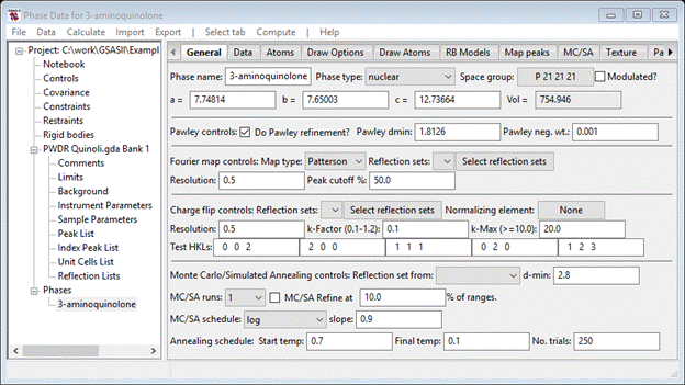
4. Go to Phases/3-aminoquinoline to find the Pawley controls under the General tab. Check the Do Pawley refinement? box, enter the d-spacing (1.8126) into the Pawley dmin box and set the Pawley neg. wt. to 0.001. This will suppress possible negative Pawley reflection intensities.
When done the General tab should look like
Next find the Data tab; it will be empty except for a single line of text. Do Edit Phase/Add powder histograms; a dialog box will appear
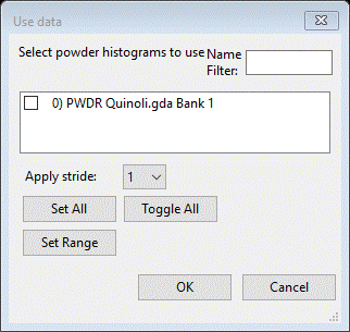
Do Set All and then OK; the desired data set will be added to this phase for analysis. The data tab now shows the new data set.
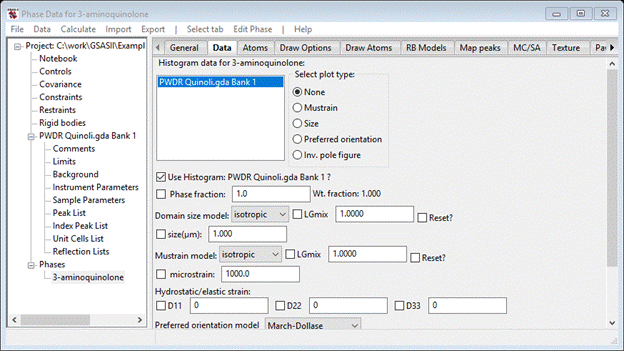
This is the location for all the phase dependent parameters for this histogram. Notice that it includes phase fraction, size & mustrain as well as preferred orientation, elastic strain and extinction corrections. The Babinet correction is intended for protein work where a significant region of the structure is disordered solvent. There are buttons for plotting size and mustrain surfaces and preferred orientation correction curves.
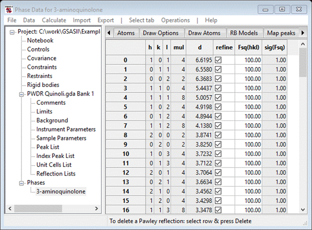
Next find the Pawley reflections tab; it will be empty except for column headings. Do Operations/Pawley create; this makes the reflection set over the range covered by setting Pawley dmin. The table should list reflections 0-91. Select and check the refine column using the same technique you used for the peak list.
This completes the Pawley refinement setup; be careful that you didn’t skip a step as it might not work correctly if you did.
Step 5. Pawley refinement
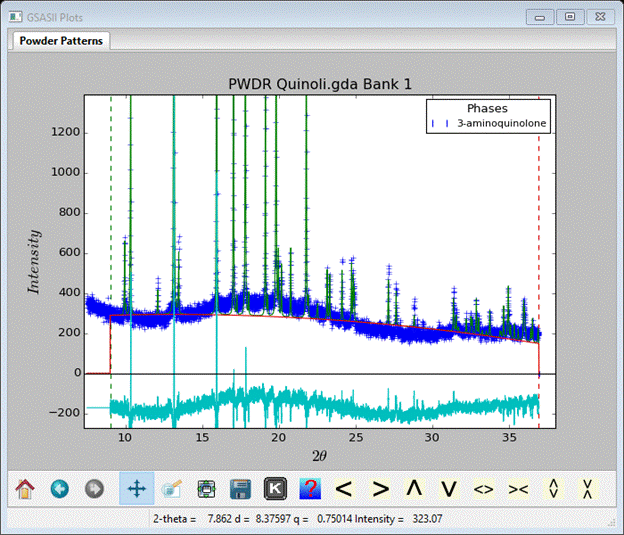
To start the refinement, do Calculate/Refine on the main GSAS-II data tree window. Before it begins a backup of the project file is made; the name will be aminoquinoline.bck0.gpx. It can be used to recover from a bad refinement. A progress dialog box will appear showing the residual as the refinement proceeds. My refinement (after 2-3 tries) completed with Rwp ~13%; a dialog box appears asking if you wish to load the result. Press OK. To see the plot select the PWDR line in the GSAS-II data tree (I’ve adjusted the width and height).
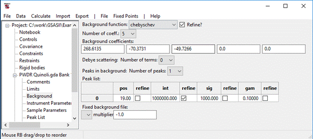
I’ve expanded the vertical scale to show the fit; it is evident from examining the plot that improvement can be had by improving the background model. One easy way to fit that broad hump is to add a peak to the background. Go to Background and set No. peaks to 1, then change pos to 19, int to 100000 and sig to 1000; for the peak only refine int. I also set No. coeff. to 5; the window shows
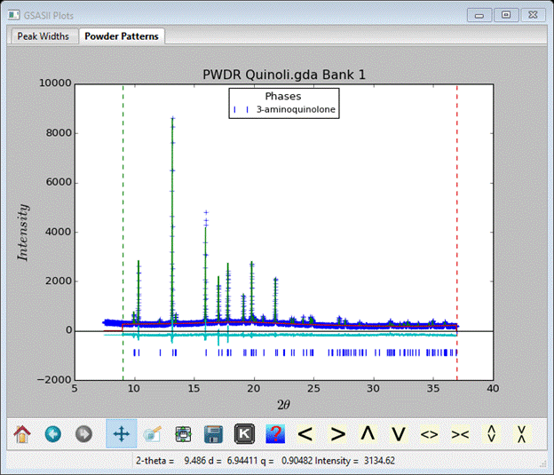
Do a Calculate/Refine; my Rwp fell to ~10%. In Background select pos & sig for refinement and in Instrument Parameters select X & Y for refinement; then do Calculate /Refine again. I got Rwp~8.3% at convergence and the fit looked like
This may be good enough to try Monte Carlo/Simulated Annealing.
Step 6. Setup for Monte Carlo/Simulated Annealing
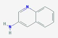
The molecular structure of 3-aminoquinoline is two aromatic rings with one N-substituted position and an amino side group
MC/SA structure solution consists of optimizing the position and orientation of this object in the unit cell; it has no internal degrees of freedom. Thus we need to determine essentially six parameters. To do this in GSAS-II we need to put a model of this molecule in as a rigid body. One must create the model outside of GSAS-II, it has no facilities for model building. I used the Avogadro (http://avogadro.cc/wiki/Main_Page) package for this and created a simple xyz Cartesian coordinate file for it (if you have Avogadro or something equivalent you can try this for yourself). To start go to Rigid bodies in the main GSAS-II data tree. You will see a window with two tabs; select Residue rigid bodies and then do Edit Body/Import XYZ. Change the file type to XYZ file (*.xyz) and select aminoquinoline.xyz. The Rigid bodies window will show
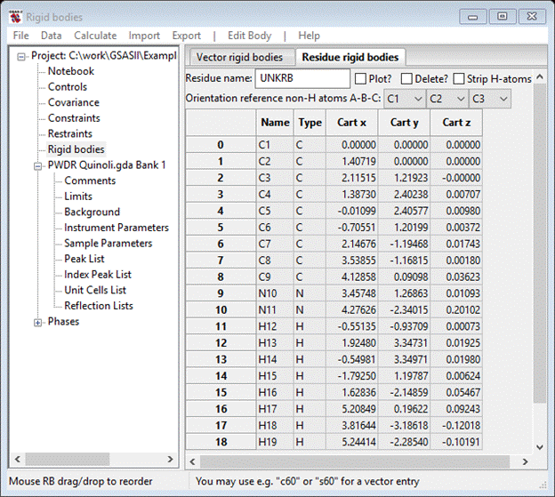
You should change the Residue name to something
meaningful, I used amino.
If you select the Plot? box a drawing will appear
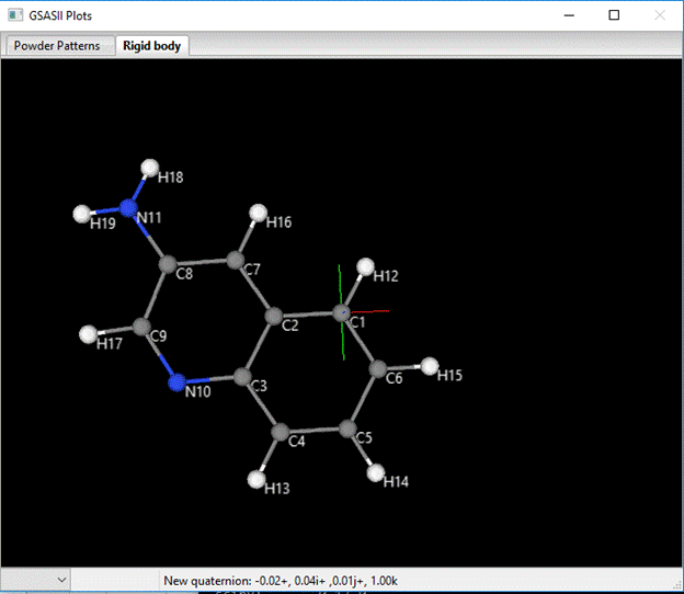
The orientation is determined by rotation and translation about a coordinate system centered on C1 and defined by the vectors C1-C2 and C1-C3. The C1-C2 vector defines the X-axis (red), the cross product of C1-C2 and C1-C3 defines the Z-axis (blue; default view direction) and the Y-axis is defined as Z-axis cross X-axis (green; down toward C5). You can change these via the pull downs next to Orientation reference non-H atoms A-B-C (you can’t pick the same atom for two of these so pick them appropriately; I chose C2, C3 & C6). At each choice the structure will be transformed accordingly. My new model is

The molecular coordinate system has been changed by you assignment of reference atoms. The C2-C3 vector is now the X-axis (red), the C2-C6 vector is ~ the Y-axis (green) and the Z-axis (blue) is ~normal to the molecular plane. The rigid body coordinates reflect this change
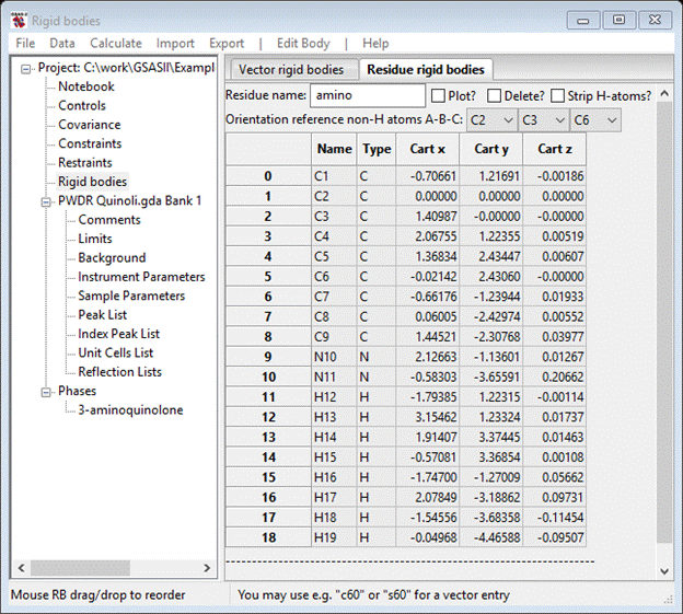
The Cart z values are all close to zero and C3 has only a nonzero Cart x. Notice that the model includes H-atoms; they are not really needed for MC/SA and will just make computation times a bit longer than necessary. They can be removed by selecting the Strip H-atoms box; for now leave them in.
Next go to Phases/3-aminoquinoline and select the MC/SA tab and do MC/SA/Add rigid body; select the only choice (amino) from the popup selection box. The MC/SA window shows
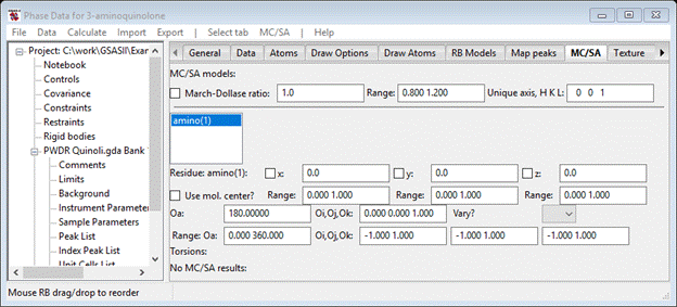
And the plot shows the molecular XYZ-axes lined up along the crystal abc-axes; this is expected from our choice of molecular reference atoms (C2, C3 & C6).
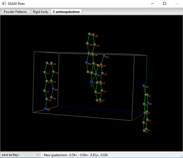
You see the four equivalent molecules for space group P212121 whose centers fall within the unit cell; the reference one is that in the lower right corner with C2 at the origin. You can enter values in the x,y,z boxes and see how the structure changes. Similarly, you can enter an angle in Oa or a vector in the Oi,Oj,Ok box to see the effects of rotating the molecule. Each of these parameters has a defined range for the MC/SA optimization run we are about to do; they define the multidimensional search volume. Within that volume will be a number of correct solutions to the structure problem all related by translational and space group symmetry. One can limit this volume by choosing more limited ranges, but here we’ll just go with the default. We want to optimize the position and orientation of this molecule; check the x, y & z boxes and select AV from the Oa, Oi,Oj,Ok Vary? pulldown. The MC/SA window should look like

This completes the set up for MC/SA processing.
Step 7. Monte Carlo/Simulated Annealing
Now go to the General tab; the MC/SA controls are at the bottom of the window. To begin the setup of these controls, select a source of the Reflection set to be used in the MC/SA runs. The choice is to use either the Pawley reflections or the Reflection List for the PWDR data set. If you choose Pawley reflections then the structure factors will be Pawley model values, Fsq(hkl) in Pawley table, and the covariance matrix developed from the refinement will be used for peak overlap effects in the MC/SA calculations. Alternatively, if you choose PWDR Quinoli.gda Bank 1 then the structure factors will be those, Fosq in Reflection table, extracted during the Pawley refinement and the peak FWHMs will be used for peak overlap effects in the MC/SA calculations. Notice that the Pawley Fsq(hkl) values are the same as the Fcsq Reflection List values. Here I chose PWDR Quinoli.gda Bank 1 for the Reflection set as it gives slightly better performance in MC/SA.
Next, you need to set the minimum d-spacing (d-min). Smaller values gives minima in the MC/SA minimization surface that are more sharply defined (thus harder to locate), while larger values yield insufficient numbers of reflections to give sufficient redundancy in the calculations. One should have 5-8 reflections for each MC/SA parameter; in this case 35-50 reflections are needed. If you examine the reflection list (either Pawley or Reflection List) you’ll see that a d-min of 2.5 will give sufficient reflections.
Lastly, you need to set the run controls. I used 500 for the No. trials; this is the number of random tries at each “temperature” in the annealing schedule. I also used 4 MC/SA runs When done the General window should look like

When ready, you can start the MC/SA calculation by doing Compute/MC/SA from the General window menu. A progress bar will appear that shows the MC/SA residual (an R-factor) as the calculation progresses through the annealing schedule as well as indicating which MC/SA run is being done. When it finishes, control is shifted to the MC/SA window which gives a list of the solutions it found at the bottom of the window (scroll down to see them).

The one with the lowest residual is already chosen and the corresponding structure is drawn

If you are lucky (like I was!) then the result is clearly a good solution with a very low Residual (~7.2%). This problem typically gives suitable solutions with Residuals of 7%; if you had stripped the H-atoms, the best residual is ~10%. If your cell indexing resulted in a & b swapped, you should view the structure along a (red). If no good solution appears (e.g. molecules clashing & high residuals), then you should just rerun MC/SA perhaps using more runs or more trials.
The MC/SA calculations can take advantage of multicore machines. First set the number of cores by doing File/Preferences; select Multiprocessing_cores from the pulldown and enter the number you wish to use (I suggest Maxcores-1). Then press Save current settings; your choice becomes available immediately and is then set for all your future uses of GSAS-II. Go to the General tab and select Compute/Multi MC/SA to use it.
Be sure to set the Keep box for any solutions you want to retain; the others will be cleared before the next MC/SA run starts. When you think you have a good one, Select it; the parameters will be copied to the appropriate boxes in the upper part of the MC/SA window and the structure is drawn again. Next we want to refine this solution so go back to the General tab.
MC/SA refinement is achieved by narrowing the search ranges and rerunning the MC/SA calculations. This is done by checking the MC/SA Refine box under the General tab. Using 10% of the ranges reduces the search volume in this case by ~6 orders of magnitude so that the true minimum is much easier to find. Now rerun Compute/MC/SA; be sure to select the best one before starting. The residual might drop to a much lower level. This refinement can be repeated with tighter restriction on the ranges. My result (no improvement on 7%) was

This is clearly a good result (R ~ 7.2%!) and the structure

Has a different origin choice (a & b might also be switched) than the published one
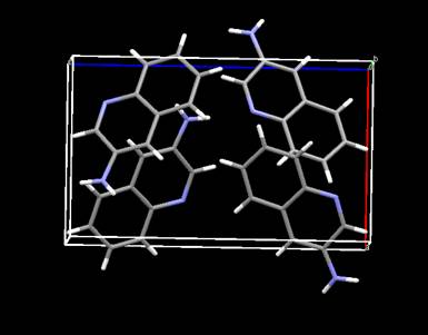
as drawn by the Mercury program
(https://www.ccdc.cam.ac.uk/Solutions/FreeSoftware/Pages/FreeMercury.aspx). To save this solution to the Atoms list do MC/SA/Move MC/SA solution; the drawing will show the new atom positions

And they will be listed in the Atoms table.

It is now ready for Rietveld refinement; this needs to use the rigid body as the data will not support independent atom position refinement.
Step 8. Initial Rietveld refinement
After a few simple steps the 3-aminoquinoline structure will be ready for the first Rietveld refinement: 1) On the General tab uncheck the Do Pawley refinement? box, 2) check the Histogram scale factor box in Sample Parameters and 3) zero both X & Y and uncheck their refine boxes in Instrument Parameters. Then do Calculate/Refine from the main GSAS-II data tree window; my Rwp was ~12%. Next check the Refine unit cell in the General window and in the Data window, using the uniaxial model for mustrain, check both Cryst. size and both mustrain boxes and do another Calculate/Refine (twice) I got an Rwp ~8.2% for this. We’ve not refined atom positions or thermal parameters; to do this we need to describe the structure as a rigid body.
Step 9. Rigid body model
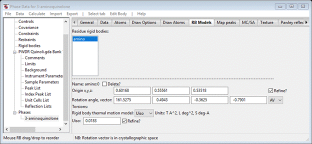
The rigid body itself has already been defined; it was used for the MC/SA structure solution. Now we have to place it in the unit cell matching the atom positions obtained from the MC/SA runs. First go to the Draw Atoms tab and change the Style to balls & sticks and the Label to name. Double click on the column headings and select the item from the popup control. Next go to the RB Models tab; it will be empty. Do Edit Body/Assign atoms to rigid body; then select amino in the Select rigid body model pull down (the only choice). The RB Models window will show
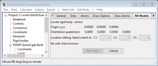
You will orient the rigid body against the atoms by matching up the 3 reference atoms in the rigid body (C1, C2 & C5) to the corresponding atoms in the structure (C(2), C(3) & C(6)). Do these in order; the drawing will show the shift of molecular origin and then its reorientation as the three atoms are selected. Press OK when done; the structure will be drawn with orange bonds indicating that it is now a rigid body and not independent atoms. The RB Models window shows the new rigid body

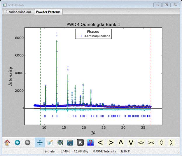
To refine the rigid body origin position check the Refine? box, select AV from the pull down, choose Uiso from the thermal parameter model and check its Refine? box. Then do Calculate/Refine; after a couple of refinement runs I got an Rwp ~7.9% and the RB Models window shows the new parameters
and the profile shows the fit
This completes the structure analysis for 3-aminoquinoline. Next is a more complex case involving some internal degrees of freedom in the molecule of a-d-lactose.